


Disclaimer
It is advised that you have a solid understanding of data structures and regular search algorithms.
Defining the Problem
To solve the problem, first, we need to have a problem.
Let's start simple. Do you know 8-puzzle? It is a really simple game. You have a 3x3 grid with 8 cells numbered from 1 to 8 and one cell blank. Your goal is to sort this mess of numbers from top left to bottom right. A blank cell will be on either end of this sorted list.
Now, we have defined a playing board, a starting state, and a goal but what about the movement set? What can we do on this playing board? Do we rip those cells out and stick them in the correct place?
Of course not. For every cell, when applicable, the only possible move is to swap the blank cell with an adjacent one. And why I said something fancy like "when applicable" is because every cell can only move in four main directions: up, down, left, right, and only within the 3x3 grid.
| 4 | 3 | 6 |
| 2 | 1 | 8 |
| 7 | - | 5 |
So now, we have a well-defined problem. Now, how the hell do we design an algorithm to solve this thing?
We will come back to this but let's step back for a second and do the hardest part first.
Naming Stuff
Let's see what we have to name. We have a starting point, the first state of the playfield. We are going to use %100 of our brainpower and call this big S.
Then we have the goal. The actual thing we are aiming for. Going above and beyond our limits, we are going to call it big G.
And, of course, we have our movement set. But possible moves change from state to state so we need to define this as a function. Because we are naming geniuses, we will call it ops(n).
Each operation is not created equal and some operations can be more costly than others. Similarly, the cost of getting to any state can be different from one other. We want to evaluate the cost of each state and because it is a function and nothing can stop us, we are going to call it f(n).
To summarize:
S = Start state
G = Goal state
ops(n) = Possible operations at any state "n"
f(n) = Evalutaion of any state "n"
Analysis
Now, since we are going to talk about multiple algorithms, we should have a way of comparing them. We will use the usual metrics and some more.
Completeness: If there is a solution, will it definitely find it?
Optimality: Is the first solution the best solution and has the least cost?
Time Complexity: Number of steps taken until solution.
Space Complexity: Memory required to run the algorithm.
And to explain time and space complexity further we are going to use:
b: Branching factor, max value of
ops(n).d: Depth of best solution.
m: Maximum depth of search space (can be infinite).
Base Algorithm
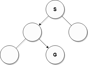
I used the word "depth" right up there. This might be confusing at first but we visualize these solutions on a tree because what we are doing looks like a decision tree. The root is S, and we have G somewhere down the line but don't know where which is the problem.
So how are we going to traverse through this tree?
First of all, we need to loop until we find G so we have the first line like this.
while G is not found:
Now we can update the current state.
Get next state
And of course, we need to check if this is G.
if the state is G, we are done here, return the solution.
But we are going to fail this check most of the time. So, we need to generate new states to see where we can go from here.
Generate new states with ops(n) from state
And we add them back to the pile.
Add new states back to the pile
Finally, we are going to define the place where algorithms separate from one another. At the start of the loop, we said Get next state but which one in the pile is the next state? This part will choose the next state.
Do magic with f(n) to choose the next state
We can sum all of this together to create our base algorithm. This will be the recurring theme for the rest of the journey. Every algorithm in the list uses this code structure with some small changes.
while G is not found:
    Get next state
    if the state is G, return the solution
    Generate new states with ops(n) from state
    Add new states back to the pile
    Do magic with f(n) to choose the next state
Blind Algorithms
What we mean by blind here is that these algorithms have no idea if they are close to the solution or not. They only know how to do one thing, and they just do it, repeatedly, until they reach the solution. This might sound like they are brute force algorithms, and in this context, yes, they are.
Breadth First Search (BFS)
I am sure we all know what BFS is but let's sum it up again.
You have a queue and you add new elements to the end of the queue and you always take the first element from the queue while searching.
I am sure the first question in your mind is, "Where the hell did queue come from, I thought we were talking about trees?". And you would be slightly incorrect. I said we visualize our work as a tree, I didn't say we use a tree. As it turns out, it is way easier to serialize these operations on a queue than on a tree.
Let's see how BFS differentiates from the base algorithm.
while G is not found:
    Get next state
    if the state is G, we are done here.
    Generate new states with ops(n) from state
    Add new states to the end of the queue
Good old BFS. Nothing special about it, really. So let's analyze it straight away.
| Completeness | Optimality | Time Complexity | Space Complexity |
| Yes | Conditional | O(b^d) | O(b^d) |
Completeness: This algorithm is complete because if there is a solution it will eventually reach it. It calculates every possible state and will eventually find G.
Optimality: This algorithm is only optimal on the condition that all possible moves have the same cost. In the case of an 8-puzzle, each move has the same cost. But if we are looking to find a path between two cities, different roads have different lengths, therefore different costs.
Complexity: Time and Space complexity go hand in hand in this as we are calculating, storing, and evaluating every possible state, and complexity grows exponentially.
This is good and all but that Optimality kinda stings the eye. Can we improve that?
Yes, we can.
Uniform Cost Search (UCS)
UCS makes a slight change to the code to achieve Optimality.
while G is not found:
    Get next state
    if the state is G, we are done here.
    Generate new states with ops(n) from state
    Add new states to the end of the queue
    Sort the queue by f(n)
Only the last line is different. By always choosing the least costly operation we can improve the algorithm.
| Completeness | Optimality | Time Complexity | Space Complexity |
| Yes | Yes | O(b^d) | O(b^d) |
Completeness: Same with BFS, this algorithm will always find G.
Optimality: Because we are working with the least cost in mind, when we find
Gwe can be sure that our solution is the best solution. There might be other solutions with the same cost but none better.Complexity: Complexity is the same as BFS because when the operation costs are the same this algorithm is the same as BFS.
This is the only Optimal algorithm we will find in the Blind Algorithms category so it is kinda special. Usually, space is the limiting factor and the problem with this algorithm.
But do you know who doesn't have a problem with space?
Depth First Search (DFS)
This is where we will see the brilliance of using queues actually. We will not implement a stack like we usually do, instead, we will make a small change to BFS and call it a day.
while G is not found:
    Get next state
    if the state is G, we are done here.
    Generate new states with ops(n) from state
    Add new states to the start of the queue
By adding new states to the start we make sure that they are retrieved first from the queue which makes up our DFS logic.
| Completeness | Optimality | Time Complexity | Space Complexity |
| Conditional | No | O(b^m) | O(b*m) |
Completeness: Unfortunately, this algorithm is susceptible to infinite loops. Two states creating each other will put this algorithm in a bugged state. And remember that
mcan also be infinite. We cannot be sure that it will find a solution unless it is a hazard-free search space.Optimality: Even when we find a solution, we cannot be sure that it is the best solution. There can be a better path to
Gthrough one of the unexplored states.Complexity: Opposite to UCS, this algorithm suffers from time constraints rather than space. Because we are exploring the visual tree as deeply as possible, time complexity scales with
minstead ofd. On the flip side, because we are not calculating and storing every single possible state, our space complexity is linear!
This algorithm shines when there isn't enough space to run other alternatives. This is one of the few linear space complexities we will see around here so it is pretty special in its own way.
But can't we do something about that infinite loop?
Iterative Deepening Search (IDS)
As the name might have suggested, IDS limits the maximum depth limit of DFS to achieve completeness.
Define max depth limit as 0
while G is not found:
    Reset to S
    Run DFS with the max depth
    Increase max depth limit
By limiting the depth of DFS, we can make sure to find a solution and can avoid infinite loops.
| Completeness | Optimality | Time Complexity | Space Complexity |
| Yes | Conditional | O(b^d) | O(b*d) |
Completeness: By descending the tree level by level, this algorithm achieves completeness. If there is a solution at any level, this algorithm will eventually reach it.
Optimality: Just like BFS, this algorithm is also only optimal if all operating costs are equal.
Complexity: Thanks to the limiter, this algorithm reaches the solution without running into the deep end of the search space. So instead of
m, this algorithm scales withd.
The limiter also has the side effect of making us evaluate the same states over and over again because we return back to our S state at the start of every loop. The S state is evaluated d + 1 times for example. Can you guess why?
Normally we would hate to go over the same states again but the extra computation load never exceeds twice the size of DFS. Because time complexity is calculated like this:
(d + 1) * b0 + d * b1 + (d - 1) * b2 + ... + b * d = O(bd)
At the cost of some time, this algorithm achieves completeness and becomes conditionally optimal. Oh, also improves the complexities compared to DFS.
But we have been running from S all this time, we have never done anything with G. Is it possible to use it?
Bidirectional Search (BDS)
While it may not be possible to implement this in every example, in examples where G can be used as an S on its own, it can provide some improvements. A good example of where it can be used is the navigation example between two cities.
The idea is to find an intersection state between S and G. The search from each end is done with BFS.
while haven't met:
    One step of BFS from S
    One step of BFS from G
| Completeness | Optimality | Time Complexity | Space Complexity |
| Yes | Conditional | O(b^d/2) | O(b^d/2) |
Completeness: Because we are using BFS, we are complete.
Optimality: Just like BFS, this algorithm is only optimal if all operating costs are equal.
Complexity: Because we are only calculating, storing, and evaluating only half of the search space for each side, we are cutting the exponential in half which helps with both time and space complexity.
Comparison
Let's break the algorithms down.
| BFS | UCS | DFS | IDS | BDS | |
| Completeness | Yes | Yes | Conditional | Yes | Yes |
| Optimality | Conditional | Yes | No | Conditional | Conditional |
| Time Complexity | O(b^d) | O(b^d) | O(b^m) | O(b^d) | O(b^d/2) |
| Space Complexity | O(b^d) | O(b^d) | O(b*m) | O(b*d) | O(b^d/2) |
BFS: While it is complete and conditionally optimal, it often struggles with time and space complexity.
UCS: This is the only fully optimal algorithm in the list and is also complete which we love but it often uses even more resources than BFS on the same problem.
DFS: Not calculating the entire state space is a huge plus with this one, only if it didn't come at the cost of optimality and completeness.
IDS: This is a clear upgrade from DFS if you don't mind spending the extra time on the problem.
BDS: On paper this might the better successor to BFS. But unfortunately, it is not always possible or plausible to backtrack from
Gon every problem.
Heuristic Algorithms
So what makes the next two algorithms heuristic? What do they know that the last five are in the dark about?
We tapped into the answer briefly with Bidirectional Search and we have actually answered it back at the start of the Blind Algorithms section. Blind algorithms have no idea if they are close to G or not. They just do the same thing over and over.
Heuristic algorithms use one more metric, something the blind algorithms don't use. It is an approximation between states and the goal. We need to know how close we are to the goal every step of the way.
Let's go over some examples. Think of a navigation system. We don't know the best path between the two cities, if we did that would be our solution. But we know the coordinates of each city and we can get a bird's eye distance between two cities as an approximation. It is easy to calculate Euclid's Distance between two points.
Or let's go back to the 8-puzzle. Think for a second that we could just rip off tiles of the board and put them in the correct place. In this case, we can define the distance between G and any state by the number of misplaced tiles at any state. Because that is how many moves we need to make to get to the goal.
Of course, this is a massive simplification of the game. This is called an optimistic approach because the new problem will always be solved with fewer moves than the real one. This works perfectly well, exactly because it is an optimistic approach, but we will come back to that later on.
Let's see what the next two algorithms do with the new information.
Best-first Search (BS)
To get to know BS better, first, we need to reevaluate our cost function. We are going to do something simple.
f(n) = h(n)
Where h(n) defines the approximate distance from the current state to G. And this will help us move in the direction of our G instead of away from it. If you want to go to a city, you drive towards it, not away from it, right?
The letter "h" also stands for "heuristic", so we still have our great naming skills in play.
while G is not found:
    Get next state
    if the state is G, return the solution
    Generate new states with ops(n) from state
    Add new states back to the queue
    Sort queue based on f(n)
The base algorithm is the same as UCS if you have been keeping track of it. The only real difference is that we are using the approximate cost until G instead of cost from S.
We seem to be always moving towards the goal. This should make the algorithm way better, right?
Well, about that...
| Completeness | Optimality | Time Complexity | Space Complexity |
| No | No | O(b^m) | O(b^m) |
Completeness: Unfortunately, this algorithm is susceptible to loops. This algorithm will jump between two states with the same distance to
Gas long as they generate one other.Optimality: Since we are working with approximate costs and not actual costs, we cannot ensure optimality.
Complexity: We store the approximate costs in memory at all times so space complexity is already high. Time-wise however, good rules and restrictions can provide a great boost to performance.
This may not look like an upgrade from something like UCS with its horrible-looking complexities but it does actually perform way better. If BS would go through as many states as UCS, it would be a horrible algorithm. But BS makes educated guesses and chooses better states, therefore, reaching the solution way faster than UCS, which cuts down the time and memory usage. It outperforms by being smarter.
Now you may ask if using approximate costs instead of real costs is the problem with lack of optimality, why not introduce it back into the algorithm? And I say, you are absolutely right, let's do that.
A* Search
We introduced these approximate costs and BS just jumped on the gun. It forgot that we still have costs to care about.
So far we have used two different f(n) functions:
f(n) = g(n)whereg(n)is the cost of any state fromS, which I didn't explicitly say for simplicity sake,And
f(n) = h(n)whereh(n)is the approximate cost untilG.
Now we are going to merge them together. Literally.
f(n) = g(n) + h(n)
The evaluation of each state is now defined by the cost to state from S plus the approximate cost to G from the state.
There are no changes to the base algorithm as we can see.
while G is not found:
    Get next state
    if the state is G, return solution
    Generate new states with ops(n) from state
    Add new states back to the queue
    Sort queue based on f(n)
We only redefined the f(n) for our needs. So let's analyze it.
| Completeness | Optimality | Time Complexity | Space Complexity |
| Yes | Conditionally | O(b^d) | O(b^d) |
Completeness: Because the infinite loops increase the
g(n), we can avoid them and find the solution.Optimality: In most cases, this algorithm is going to be optimal. But to ensure that, we must fulfill a condition which we will talk about in the next section.
Complexity: Same as BS. We store the approximate costs in memory at all times and space complexity scales exponentially. Time-wise, good rules, and restrictions can provide a great boost to performance.
Funny enough, A* usually works as fast as BS if not better. So space and time complexity doesn't reach ridiculous numbers but this doesn't mean they are immune to these problems either. Long-winded problems will require a great deal of memory and tricky ops(n) will be taxing time-wise.
Optimality of A*
The short answer is for h(n) to be optimistic. We want the approximate cost of any state to be lower than the actual cost of the state.
Let's explain with an example. Assume the following:
h(n)is optimistic,GandG2are the goal states,Gis the optimal solution with the least cost,G2is a sub-optimal solution with a higher cost,States
nandG2are in the queue,We need to choose the next state to take out from the queue.
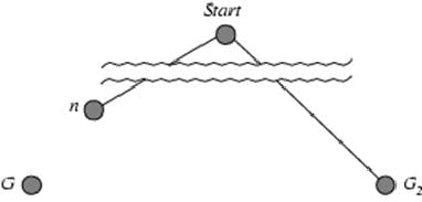
If we take out G2 first, our algorithm will never be optimal, but if we can prove that the algorithm will always choose n over G2 then we can call it optimal.
So, let's do some math.
f(G2) = g(G2)   // Cost h(G2) is 0.
f(G) = g(G)     // Cost h(G) is 0.
g(G) < g(G2)    // Becuase G2 is not optimal.
f(G) < f(G2)    // Based on last three lines.


h(n) =< *h(n)                // Where *h defines the real cost.
g(n) + h(n) =< g(n) + *h(n)  // Add g(n) to both sides.
f(n) =< f(G)                 // Because h(n) is optimistic and real costs sum up to f(G).
f(n) =< f(G) < f(G2)         // Because f(G) < f(G2).
f(n) < f(G2)                 // The solution
And because A* always takes out the least costly state from the queue we can safely say that, when h(n) is an optimistic approach to the problem, the A* algorithm is an optimal algorithm.
How did we get here?
The long way around, I guess. But we are here because A* is everywhere. We generally use it on pathfinders in navigation systems, cleaning bots, and game AIs. And it also finds use in parsing using stochastic grammar in Natural Language Processing.
And also I may have written a 4000-word document on search algorithms because someone talked about A* for like an hour two weeks back and I can't get it out of my head. Yeah, I think I know how we got here.
I also know where we need to go next. We need to code this thing out. So... Get on with it.